An ideal read for ML practitioners venturing into Neural Networks for the first time. A basic tutorial of implementing Neural Networks from scratch, bridging the gap between the reader’s ML knowledge and the Neural Network concepts. The time is ripe to enhance your ML expertise!
A few days back I started learning Neural Networks, before that I had a basic knowledge of Machine Learning. So, I think this is the best time to write this article for those who know ML and are hoping to start learning Neural Networks. I have found these techniques useful to learn NN from the mind of a person who knows ML priorly. I have explained the concepts in a way that you can relate them with the concepts of ML, and it will be a very quick journey for you to learn these concepts quickly and easily.
This post will guide you through implementing a basic neurons, then combining those neurons to form layers and finally combining layers to make Neural Networks.
Let’s get Started ! 🏁
To start this awesome journey, let’s first quickly revise some concepts of ML… this is the time to recall them and prepare your mind to get started.
ML recall 💡
The only concept that you need to remember to get this article in your is of Linear Regression!.
Here are the steps that we follow in Linear Regression :
Get a tabular that we want to train.
Separate the data in two parts, Independent and Dependent Variables. \[[x_1^1, x_2^1, x_3^1, x_4^1, x_5^1...] , [y_1]\]\[[x_1^2, x_2^2, x_3^2, x_4^2, x_5^2...] , [y_2]\]\[[x_1^3, x_2^3, x_3^3, x_4^3, x_5^3...] , [y_3]\]\[.....\]
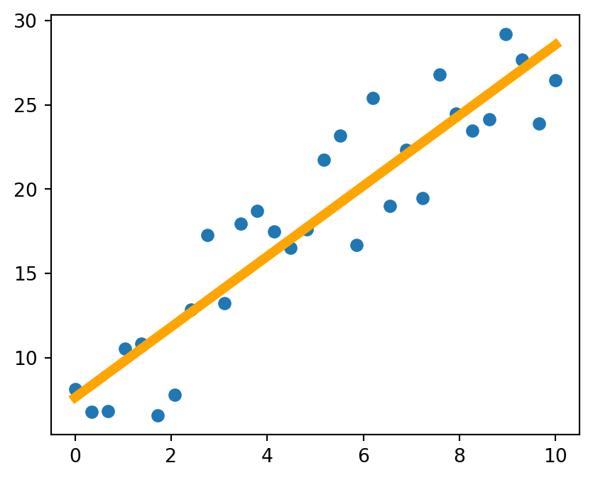
The equation to fit the line is …
\[y = mX + b\]
Loss Function used can be root-mean-square error… \[RMSE = \sum_{i=1}^{D}(y_i-(mX_i + b))^2\]
Now we find a best-fit line that fits the data with minimum loss. We do this with the help of gradient descent (reducing the loss in every step by modifying the weights)
And so, this is all you need to know to get started ! So, now lets dive deep into implementation of NN from scratch.
Know some Tensors 🍃
Tensors are a fundamental data structure, very similar to arrays and matrices. A tensor can be represented as a matrix, but also as a vector, a scalar, or a higher-dimensional array.
tensor are just like numpy arrays and so, there is not much to think about them, lets get to the next big thing…
Designing your first neuron ⚛️
A single neuron (or perceptron) is the basic unit of a neural network…
It takes input as dependent variables, multiplies it with the weights, adds the bias , goes through an activation function, and produces the output.
I know what you are thinking now 👀…
Huh! It looks the same as Linear Regression Model !!
😌 Yes, it is just another Linear Regression .
Then what is that activation function?
😌 This is something you will get to know in the near future.
Should I relax?
😌 Absolutely NOT !!
A Perceptron
So, Let’s implement this using tensor
Data Preprocessing (can be skipped)
The data used for this e.g. is the most famous, Titanic Dataset. Some preprocessing steps are done (you might be familiar with them and so, they can be skipped)
Code
# Some Data Cleaning and Preprocessingdf = pd.read_csv('train.csv') # read datasetmode = df.mode(axis=0,).iloc[0] # calculating mode of all columnsdf.fillna(mode, inplace=True) # filling missing values with modedf['FareLog'] = np.log(df['Fare'] +1) # taking log of fare ( feature engineering )cat_cols = ['Sex', 'Pclass', 'Embarked'] # category columnsdf_cat = pd.get_dummies(df, columns=cat_cols) # transforming categories to numerical valuesindep_cols = ['Age', 'SibSp', 'Parch', 'FareLog', 'Pclass_1', 'Pclass_2', 'Pclass_3','Sex_female', 'Sex_male', 'Embarked_C', 'Embarked_Q', 'Embarked_S','Embarked_S'] # list of independent columns dep_cols = ['Survived'] # list of dependent columnsdf = df_cat[indep_cols + dep_cols] # final dataset
df.head(2)
Age
SibSp
Parch
FareLog
Pclass_1
Pclass_2
Pclass_3
Sex_female
Sex_male
Embarked_C
Embarked_Q
Embarked_S
Embarked_S
Survived
0
22.0
1
0
2.110213
False
False
True
False
True
False
False
True
True
0
1
38.0
1
0
4.280593
True
False
False
True
False
True
False
False
False
1
Set X and Y tensors
The Survived value is what we have to predict. And instead of using pandas or numpy, we are using tensor.
Initialize the values of dependent and independent variables as tensors like this…
X = tensor(df[indep_cols].values.astype(float))y = tensor(df[dep_cols].values.astype(float))max_val, idxs = X.max(dim=0)X = X / max_val
X.shape :  torch.Size([891, 15])
y.shape :  torch.Size([891, 1])

First Row of X :
tensor([0.2750, 0.1250, 0.0000, 0.3381, 0.0000, 0.0000, 1.0000, 0.0000, 1.0000,
        0.0000, 0.0000, 1.0000, 1.0000, 1.0000, 1.0000], dtype=torch.float64)

First Row of y :
tensor([0.], dtype=torch.float64)
Initialize the weights
We have to make a weights tensor that will be used as coefficients. At the start of training, it can be a random valued tensor, we can design a function for this… To keep it simple initially, we are not using bias term rn.
torch.rand() takes the shape of required tensor and generates it
Very similar to Linear Regression, Predictions can be calculated by the weighted sum of features and weights. For loss, we have used Mean Absolute Error…
Now,as we have all the necessary functions, we can perform our first epoch, a single epoch will calculate the loss, takes the gradient value according to learning rate and modify the coefficients to reduce the error. This is exactly same as a single step of gradient descent…
\[Weight = Weight - LearningRate * Gradient\]
def update_coeff(coeff, lr):# subtracts the value from coeff and save it as a new value coeff.sub_(coeff.grad * lr) coeff.grad.zero_() # sets the coeff.grad value to 0
flowchart LR
  A[Random Weight] --> B(Calculate \nLoss)
  B --> C(Calculate \nGradient) --> D(Modify\n Weights)-->|for n epochs|B
  D --> E[Final Weights]
def one_epoch(coeff, lr): loss = calc_loss(coeff, X, y) loss.backward() # new term alert !print(f' loss : {loss:.3} ', end=';')with torch.no_grad(): # no_grad mode update_coeff(coeff, lr)def train_model(n_epochs, lr): torch.manual_seed(442) coeff = init_coeff(X) coeff.requires_grad_() # new term alert !for i inrange(n_epochs): one_epoch(coeff, lr)print('\n\nFinal Loss: ', float(calc_loss(coeff, X, y)))return coeff
Autograd Mechanism ⚠️
coeff.requires_grad_() sets the value of coeff.requires_grad = True… when this is set true, the gradients values are computed for these tensors, which can be used afterward in backpropagation. So, when a back pass is done, their .grad values update with new gradient values.
loss.backward() is a back pass here. When calculations are performed (in forward pass), an operation is recorded in backward graph when at least one of its input tensors requires gradient. And when we call loss.backward(), leaf tensors with .requires_grad = True will have gradients accumulated to their .grad fields.
So, We calculate gradients by forward and backward propagation. We first set the coeff.requires_grad = True then the loss is calculated for the coeff. As coeff requires grad so, this operation will be added in backward graph. And now, when we call loss.backward(), it calculates the .grad values of all those tensors which requires grad and are in the backward graph. So, the coeff tensor will have its .grad value updated.
Then we update the coeff value. While doing this, we don’t want this operation to be saved in backward graph so, we keep this modification under torch.no_grad() function, and so, this operation is neglected and is not tracked. Next when again loss is calculated and backward fun. called, new grad values gets updated…. and the process carries on.
coeff = train_model(40,0.1)
 loss : 0.718 ; loss : 0.68 ; loss : 0.658 ; loss : 0.638 ; loss : 0.618 ; loss : 0.599 ; loss : 0.581 ; loss : 0.562 ; loss : 0.543 ; loss : 0.525 ; loss : 0.506 ; loss : 0.488 ; loss : 0.469 ; loss : 0.451 ; loss : 0.433 ; loss : 0.415 ; loss : 0.397 ; loss : 0.379 ; loss : 0.362 ; loss : 0.345 ; loss : 0.33 ; loss : 0.317 ; loss : 0.306 ; loss : 0.296 ; loss : 0.289 ; loss : 0.29 ; loss : 0.287 ; loss : 0.304 ; loss : 0.268 ; loss : 0.279 ; loss : 0.276 ; loss : 0.291 ; loss : 0.274 ; loss : 0.288 ; loss : 0.276 ; loss : 0.285 ; loss : 0.28 ; loss : 0.285 ; loss : 0.283 ; loss : 0.287 ;

Final Loss:  0.2839040984606188
Activation Function 🍭
Here we have used another function torch.sigmoid() over the calculated predictions, which is known as Activation Function!. We know that the weighted sum can produce the values less than 0 or more than 1. But our y has values only between 0 and 1. so, to restrict the values, we use the sigmoid function… which you might be familiar with if you know Logistic Regression.
 loss : 0.562 ; loss : 0.33 ; loss : 0.311 ; loss : 0.307 ; loss : 0.305 ; loss : 0.304 ; loss : 0.302 ; loss : 0.3 ; loss : 0.292 ; loss : 0.234 ; loss : 0.217 ; loss : 0.215 ; loss : 0.214 ; loss : 0.212 ; loss : 0.21 ; loss : 0.206 ; loss : 0.203 ; loss : 0.201 ; loss : 0.2 ; loss : 0.199 ; loss : 0.198 ; loss : 0.197 ; loss : 0.197 ; loss : 0.196 ; loss : 0.196 ; loss : 0.196 ; loss : 0.195 ; loss : 0.195 ; loss : 0.195 ; loss : 0.195 ; loss : 0.195 ; loss : 0.194 ; loss : 0.194 ; loss : 0.194 ; loss : 0.194 ; loss : 0.194 ; loss : 0.194 ; loss : 0.194 ; loss : 0.193 ; loss : 0.193 ;

Final Loss:  0.1931743193621472
Congratulations !! You have trained your first Neuron !!!!!
Building a Layer of NN 🪵
A single layerd NN will just contain more than one Neurons as the layer. Each neuron will receive all features values and gives an output. The outputs of all the neurons of the layer will be passed to output neuron, which will combine them to produce the final output.
The first layer neurons will have weights equal to size of input features. The output neuron will contain the weights of size of no. of neurons in first layer.
Simple !!! Take a look at hidden neuron = 2 and with hidden neuron = 1
flowchart TD
  A((1)) --> Z((F))
  B((2)) --> Z
  Z --> V((Z))
  AA((I1)) --> A
  AB((I2)) --> A
  AB --> B
  AC((I3)) --> A
  AC --> B
  AD((I4)) --> A
  AD --> B
  AA --> B
  A1((1)) --> Z1((F))
  Z1 --> V1((Z))
  AA1((I1)) --> A1
  AB1((I2)) --> A1
  AC1((I3)) --> A1
  AD1((I4)) --> A1
So I1 - I4 are input features, 1 and 2 are the neurons of first layer, `
Fis the output neuron, which takes1and2` as input.
Finally Z is the activation function.
Initialization of Weights…
the weights will contain layer_1 of shape (n_coeff, n_hidden), so it will contain n_hidden set of weights, where the shape of each weight set will be of size n_coeff (input features).
And layer_2 will have 1 set of weights where the weight set will be of size n_hidden. const is the bias term added.
The predictions of hidden layer are calculated by matmul() fun for weighted sum by matrix multiplication, the activation function used for first layer is ReLu Activation Function. It is a simpler function, which sets any -ve value to 0. \[Relu(z) = max(0, z)\] The output of first layer is given input for second layer and so, is multiplied with layer2 and const term is added. The final output layer uses the sigmoid function. No change required in Loss Function
 loss : 0.518 ; loss : 0.467 ; loss : 0.44 ; loss : 0.423 ; loss : 0.412 ; loss : 0.405 ; loss : 0.399 ; loss : 0.394 ; loss : 0.386 ; loss : 0.365 ; loss : 0.298 ; loss : 0.295 ; loss : 0.333 ; loss : 0.323 ; loss : 0.317 ; loss : 0.309 ; loss : 0.27 ; loss : 0.229 ; loss : 0.226 ; loss : 0.224 ; loss : 0.221 ; loss : 0.217 ; loss : 0.212 ; loss : 0.208 ; loss : 0.207 ; loss : 0.209 ; loss : 0.203 ; loss : 0.202 ; loss : 0.199 ; loss : 0.198 ; loss : 0.197 ; loss : 0.196 ; loss : 0.196 ; loss : 0.195 ; loss : 0.195 ; loss : 0.195 ; loss : 0.194 ; loss : 0.194 ; loss : 0.194 ; loss : 0.194 ;

Final Loss:  0.19344465494371008
Building a Complete Neural Network 🔮
A complete NN will contain several layers, with different sizes. Each layer will have some perceptrons, and perceptrons of a layer will have weights of size equal to no. of perceptron in previous layer.
So, there can be any number of neurons in a layer but, they all will receive output of the previous layer and so their weights should match.
For eg, if a neural network has the following layers :
Input Layer - 3 inputs
Hidden Layers -
Layer 1 - 2 perceptrons —> (3 weights in every perceptron)
Layer 2 - 2 perceptrons —> (2 weights in each perceptron)
Output Layer - 1 perceptron —> (2 weights in each perceptron)
And, so here we have a complete neural network…!!
flowchart LR
  A1((L1)) --> Z1((L2))
  Z1 --> V1((Z))
  AA1((I1)) --> A1
  AA1 --> B((L1))
  AB1((I2)) --> A1
  AB1 --> B
  AC1((I3)) --> A1
  AC1 --> B
  B --> Z1
  B --> Z2
  A1 --> Z2((L2))
  Z2 --> V1
  V1 --> AL(OUTPUT)
Weights Initialization can contain a list of layers size as input and so it will return the coefficients and bias matrix for all layers.
def init_coeffs(n_hidden: list, indep_var): n_coeff = indep_var.shape[1] sizes = [n_coeff] + n_hidden + [1] # inputs, hidden, output n =len(sizes) layers = [(torch.rand(sizes[i], sizes[i+1]).double() -0.5)/sizes[i+1]*4for i inrange(n-1)] consts = [((torch.rand(1,1) -0.5) *0.1).double() for i inrange(n-1)]for l in (layers + consts) : l.requires_grad_()return layers, consts
- 0.5, * 0.1, * 4… and all these we only do for initial setup so that the random coeff. generated can be close to the optimum value in the start, (helpful for quickly converging the loss)
And here we can first layer has 4 perceptrons with 15 weights each, 2nd layer has 2 perceptrons with 4 weights each, output layer has 1 perceptron with 2 weights, and all the layers have 1 bias term each
Calculating Predictions requires a slight change, looping over all layers, multiply the input values with weights of each layer.
\[output = input * weights + bias\]
def calc_preds(coeff, indep_var): layers, consts = coeff n =len(layers) res = indep_varfor i, l inenumerate(layers[: -1]): res = F.relu( res.matmul(layers[i]) + consts[i] )# relu activation for all hidden layers res = res.matmul(layers[-1]) + consts[-1]return torch.sigmoid(res) # sigmoid for the output layer
Updating Coefficients will simply loop over all coeff and biases and subtracting \(gradient * learningRate\)
 loss : 0.495 ; loss : 0.436 ; loss : 0.367 ; loss : 0.353 ; loss : 0.335 ; loss : 0.316 ; loss : 0.307 ; loss : 0.307 ; loss : 0.305 ; loss : 0.267 ; loss : 0.261 ; loss : 0.237 ; loss : 0.228 ; loss : 0.223 ; loss : 0.225 ; loss : 0.213 ; loss : 0.212 ; loss : 0.214 ; loss : 0.204 ; loss : 0.202 ; loss : 0.201 ; loss : 0.2 ; loss : 0.199 ; loss : 0.199 ; loss : 0.198 ; loss : 0.197 ; loss : 0.196 ; loss : 0.195 ; loss : 0.194 ; loss : 0.194 ; loss : 0.193 ; loss : 0.193 ; loss : 0.193 ; loss : 0.192 ; loss : 0.192 ; loss : 0.192 ; loss : 0.192 ; loss : 0.192 ; loss : 0.191 ; loss : 0.191 ;

Final Loss:  0.19121552750666765
Tada 🎉🎉🎉 !!!
Now you know how to build a complete Neural Network from scratch !!!
Let me know if I missed something. 😉
Where to go from here?
😏 Haah! Nowhere !!!
PS :
For the flowcharts, I have used the tool named mermaid, you can generate them easily in markdown.
To transform this notebook into webpage, I have used Quarto.
My only recommendation - do fast.ai course 😌
Source Code
---author: Rohan Sharmadate: 10/24/2023format: html: code-fold: false code-tools: true toc: truetitle: Neural Networks From Scratch -- ML practitioner's guidejupyter: python3categories: ['Deep Learning', 'Neural Networks', 'Pytorch']------An ideal read for ML practitioners venturing into Neural Networks for the first time. A basic tutorial of implementing Neural Networks from scratch, bridging the gap between the reader's ML knowledge and the Neural Network concepts. The time is ripe to enhance your ML expertise!A few days back I started learning Neural Networks, before that I had a basic knowledge of Machine Learning. So, I think this is the best time to write this article for those who know ML and are hoping to start learning Neural Networks. I have found these techniques useful to learn NN from the mind of a person who knows ML priorly.I have explained the concepts in a way that you can relate them with the concepts of ML, and it will be a very quick journey for you to learn these concepts quickly and easily. This post will guide you through implementing a basic neurons, then combining those neurons to form layers and finally combining layers to make Neural Networks. # Let's get Started ! 🏁To start this awesome journey, let's first quickly revise some concepts of ML... this is the time to recall them and prepare your mind to get started. ### ML recall 💡The only concept that you need to remember to get this article in your is of **Linear Regression!**. Here are the steps that we follow in Linear Regression : 1. Get a tabular that we want to train.2. Separate the data in two parts, *Independent* and *Dependent Variables*. $$[x_1^1, x_2^1, x_3^1, x_4^1, x_5^1...] , [y_1]$$ $$[x_1^2, x_2^2, x_3^2, x_4^2, x_5^2...] , [y_2]$$ $$[x_1^3, x_2^3, x_3^3, x_4^3, x_5^3...] , [y_3]$$ $$.....$$3. The equation to fit the line is … $$y = mX + b$$4. Loss Function used can be root-mean-square error... $$RMSE = \sum_{i=1}^{D}(y_i-(mX_i + b))^2$$5. Now we find a best-fit line that fits the data with minimum loss. We do this with the help of gradient descent (reducing the loss in every step by modifying the weights)```{python}#| echo: falseimport pandas as pdimport numpy as npimport matplotlib.pyplot as pltimport torchx = np.linspace(0,10,30).reshape(-1,1)y = (2*x +3+ np.random.rand(*x.shape)*10).reshape(-1,1)``````{python}#| code-fold: true#| label: fig-limit#| fig-cap: linear regressionplt.figure(figsize=(5,4))plt.scatter(x,y, label='data points')from sklearn.linear_model import LinearRegressionpred = LinearRegression().fit(x,y).predict(x)plt.plot(x,pred, color='orange', linewidth=5, label='best-fit')# plt.legend()plt.show()```And so, this is all you need to know to get started ! So, now lets dive deep into implementation of NN from scratch. ## Know some Tensors 🍃Tensors are a fundamental data structure, very similar to arrays and matrices.A tensor can be represented as a matrix, but also as a vector, a scalar, or a higher-dimensional array. ```{python}from torch import tensor``````{python}np_array = np.array([[2,5,7,2],[2,6,8,3]])one_d = tensor([1,4,5,6])two_d = tensor(np_array)print(one_d);print(two_d);````tensor` are just like `numpy arrays` and so, there is not much to think about them, lets get to the next **big** thing...# Designing your first neuron ⚛️A **single neuron (or perceptron)** is the basic unit of a neural network... It takes <u>*input*</u> as <u>*dependent variables*</u>, multiplies it with the <u>*weights*</u>, adds the <u>*bias*</u> , goes through an <u>*activation function*</u>, and produces the <u>*output*</u>. I know what you are thinking now 👀... 1. Huh! It looks the same as Linear Regression Model !! 😌 Yes, it is just another Linear Regression . 2. Then what is that *activation function*? 😌 This is something you will get to know in the near future.3. Should I relax? 😌 Absolutely NOT !!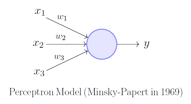So, Let's implement this using `tensor`### Data Preprocessing (can be skipped)The data used for this e.g. is the most famous, Titanic Dataset. Some preprocessing steps are done (you might be familiar with them and so, they can be skipped)```{python}#| code-fold: true# Some Data Cleaning and Preprocessingdf = pd.read_csv('train.csv') # read datasetmode = df.mode(axis=0,).iloc[0] # calculating mode of all columnsdf.fillna(mode, inplace=True) # filling missing values with modedf['FareLog'] = np.log(df['Fare'] +1) # taking log of fare ( feature engineering )cat_cols = ['Sex', 'Pclass', 'Embarked'] # category columnsdf_cat = pd.get_dummies(df, columns=cat_cols) # transforming categories to numerical valuesindep_cols = ['Age', 'SibSp', 'Parch', 'FareLog', 'Pclass_1', 'Pclass_2', 'Pclass_3','Sex_female', 'Sex_male', 'Embarked_C', 'Embarked_Q', 'Embarked_S','Embarked_S'] # list of independent columns dep_cols = ['Survived'] # list of dependent columnsdf = df_cat[indep_cols + dep_cols] # final dataset``````{python}df.head(2)```### Set X and Y tensorsThe `Survived` value is what we have to predict. And instead of using `pandas` or `numpy`, we are using `tensor`.Initialize the values of dependent and independent variables as tensors like this...```{python}X = tensor(df[indep_cols].values.astype(float))y = tensor(df[dep_cols].values.astype(float))max_val, idxs = X.max(dim=0)X = X / max_val ``````{python}#| echo: falseprint('X.shape : ', X.shape)print('y.shape : ', y.shape)print('\nFirst Row of X :')print(X[0])print('\nFirst Row of y :')print(y[0])```#### Initialize the weightsWe have to make a weights tensor that will be used as *coefficients*. At the start of training, it can be a random valued tensor, we can design a function for this… To keep it simple initially, we are not using bias term rn.`torch.rand()` takes the shape of required tensor and generates it ```{python}def init_coeff(indep_var): n_coeffs = indep_var.shape[1]return (torch.rand(n_coeffs) -0.5)```` - 0.5 ` is done to normalize the values```{python}#| echo: false# c,b = init_coeff(X)# print('Coffecients: \n', c[:,0])# print('\nbias: ', b)```#### Calculate Predictions and LossVery similar to Linear Regression, Predictions can be calculated by the *weighted sum* of *features* and *weights*.For *loss*, we have used *Mean Absolute Error…*Let's make a function for this... ```{python}def calc_preds(coeff, indep_var):return (indep_var*coeff).sum(axis=1)[:,None] def calc_loss(coeff, indep_var, dep_var):return torch.abs(calc_preds(coeff, indep_var) - dep_var).mean()```#### Epochs Now,as we have all the necessary functions, we can perform our first epoch, a **single epoch** will calculate the loss, takes the gradient value according to learning rate and modify the coefficients to reduce the error. This is exactly same as a single step of gradient descent...$$Weight = Weight - LearningRate * Gradient$$```{python}def update_coeff(coeff, lr):# subtracts the value from coeff and save it as a new value coeff.sub_(coeff.grad * lr) coeff.grad.zero_() # sets the coeff.grad value to 0``````{mermaid}flowchart LR A[Random Weight] --> B(Calculate \nLoss) B --> C(Calculate \nGradient) --> D(Modify\n Weights)-->|for n epochs|B D --> E[Final Weights]``````{python}def one_epoch(coeff, lr): loss = calc_loss(coeff, X, y) loss.backward() # new term alert !print(f' loss : {loss:.3} ', end=';')with torch.no_grad(): # no_grad mode update_coeff(coeff, lr)def train_model(n_epochs, lr): torch.manual_seed(442) coeff = init_coeff(X) coeff.requires_grad_() # new term alert !for i inrange(n_epochs): one_epoch(coeff, lr)print('\n\nFinal Loss: ', float(calc_loss(coeff, X, y)))return coeff```### Autograd Mechanism ⚠️`coeff.requires_grad_()` sets the value of `coeff.requires_grad` = `True`... when this is set true, the gradients values are computed for these tensors, which can be used afterward in backpropagation. So, when a *back pass* is done, their `.grad` values update with new gradient values. `loss.backward()` is a *back pass* here. When calculations are performed (in forward pass), an operation is recorded in backward graph when at least one of its input tensors requires gradient. And when we call `loss.backward()`, leaf tensors with `.requires_grad = True` will have gradients accumulated to their `.grad` fields.So, We calculate gradients by forward and backward propagation. We first set the `coeff.requires_grad = True` then the loss is calculated for the `coeff`. As coeff requires grad so, this operation will be added in backward graph. And now, when we call `loss.backward()`, it calculates the `.grad` values of all those tensors which requires grad and are in the backward graph. So, the coeff tensor will have its `.grad` value updated. Then we update the `coeff` value. While doing this, we don't want this operation to be saved in backward graph so, we keep this modification under `torch.no_grad()` function, and so, this operation is neglected and is not tracked. Next when again loss is calculated and backward fun. called, new grad values gets updated.... and the process carries on.```{python}coeff = train_model(40,0.1)```### Activation Function 🍭Here we have used another function `torch.sigmoid()` over the calculated predictions, which is known as **Activation Function!**.We know that the weighted sum can produce the values less than 0 or more than 1. But our `y` has values only between 0 and 1. so, to restrict the values, we use the *sigmoid* function... which you might be familiar with if you know Logistic Regression. $$\sigma(z) = \frac{1} {1 + e^{-z}}$$```{python}def calc_preds(coeff, indep_var): reg_pred = (indep_var*coeff).sum(axis=1)[:,None]return torch.sigmoid(reg_pred)``````{python}coeff = train_model(40,50)```**Congratulations !! You have trained your first Neuron !!!!!**# Building a Layer of NN 🪵A single layerd NN will just contain more than one Neurons as the layer. Each neuron will receive all features values and gives an output. The outputs of all the neurons of the layer will be passed to output neuron, which will combine them to produce the final output. The first layer neurons will have weights equal to size of input features. The output neuron will contain the weights of size of no. of neurons in first layer. Simple !!! Take a look at hidden neuron = 2 and with hidden neuron = 1```{mermaid}flowchart TD A((1)) --> Z((F)) B((2)) --> Z Z --> V((Z)) AA((I1)) --> A AB((I2)) --> A AB --> B AC((I3)) --> A AC --> B AD((I4)) --> A AD --> B AA --> B A1((1)) --> Z1((F)) Z1 --> V1((Z)) AA1((I1)) --> A1 AB1((I2)) --> A1 AC1((I3)) --> A1 AD1((I4)) --> A1```So `I1 - I4` are input features, `1` and `2` are the neurons of first layer, `F` is the output neuron, which takes `1` and `2` as input. Finally `Z` is the activation function. **Initialization of Weights...**the weights will contain `layer_1` of shape (n_coeff, n_hidden), so it will contain n_hidden set of weights, where the shape of each weight set will be of size n_coeff (input features).And `layer_2` will have 1 set of weights where the weight set will be of size n_hidden. `const` is the bias term added. ```{python}def init_coeffs(n_hidden, indep_var): n_coeff = indep_var.shape[1] layer1 = ((torch.rand(n_coeff, n_hidden) -0.5) / n_hidden).double().requires_grad_() # shape of (n_coeff, n_hidden) layer2 = ((torch.rand(n_hidden, 1)) -0.3).double().requires_grad_() # output layer, shape of (n_hidden, 1) const = ((torch.rand(1, 1)-0.5).double() *0.1).requires_grad_()return layer1, layer2, constcoeff = init_coeffs(2, X)```**Calculate Predictions and Loss**The predictions of hidden layer are calculated by `matmul()` fun for weighted sum by matrix multiplication, the *activation function* used for first layer is **ReLu Activation Function**. It is a simpler function, which sets any -ve value to 0. $$Relu(z) = max(0, z)$$The output of first layer is given input for second layer and so, is multiplied with layer2 and const term is added. The final output layer uses the **sigmoid** function. No change required in Loss Function```{python}import torch.nn.functional as F``````{python}def calc_preds(coeff, indep_var): layer1, layer2, const = coeff op1 = F.relu(indep_var.matmul(layer1)) # new term alert op2 = op1.matmul(layer2) + constreturn torch.sigmoid(op2)```**Update Coefficient** requires just a slight change, instead of single coeff, we have multiple coeff (`layer1, layer2, coeff`), so loop over all of them ```{python}def update_coeff(coeff, lr):for layer in coeff: layer.sub_(layer.grad * lr) layer.grad.zero_()```**Train Function** requires a slight change to give `n_hidden` value as input for init_coeff()```{python}def train_model(n_epochs, lr, n_hidden=2): coeff = init_coeffs(n_hidden, X)for i inrange(n_epochs): one_epoch(coeff, lr)print('\n\nFinal Loss: ', float(calc_loss(coeff, X, y)))return coeff``````{python}coeff = train_model(40,10)```# Building a Complete Neural Network 🔮A complete NN will contain several layers, with different sizes. Each layer will have some perceptrons, and perceptrons of a layer will have weights of size equal to no. of perceptron in previous layer. So, there can be any number of neurons in a layer but, they all will receive output of the previous layer and so their weights should match.For eg, if a neural network has the following layers : - *Input Layer* - 3 inputs- *Hidden Layers* - - Layer 1 - 2 perceptrons ---> (3 weights in every perceptron) - Layer 2 - 2 perceptrons ---> (2 weights in each perceptron)- *Output Layer* - 1 perceptron ---> (2 weights in each perceptron)*And, so here we have a complete neural network...!!*```{mermaid}flowchart LR A1((L1)) --> Z1((L2)) Z1 --> V1((Z)) AA1((I1)) --> A1 AA1 --> B((L1)) AB1((I2)) --> A1 AB1 --> B AC1((I3)) --> A1 AC1 --> B B --> Z1 B --> Z2 A1 --> Z2((L2)) Z2 --> V1 V1 --> AL(OUTPUT)```**Weights Initialization** can contain a `list` of layers size as input and so it will return the coefficients and bias matrix for all layers. ```{python}def init_coeffs(n_hidden: list, indep_var): n_coeff = indep_var.shape[1] sizes = [n_coeff] + n_hidden + [1] # inputs, hidden, output n =len(sizes) layers = [(torch.rand(sizes[i], sizes[i+1]).double() -0.5)/sizes[i+1]*4for i inrange(n-1)] consts = [((torch.rand(1,1) -0.5) *0.1).double() for i inrange(n-1)]for l in (layers + consts) : l.requires_grad_()return layers, consts````- 0.5`, `* 0.1`, `* 4`... and all these we only do for initial setup so that the random coeff. generated can be close to the optimum value in the start, (helpful for quickly converging the loss)```{python}[x.shape for x in init_coeffs([4, 2], X)[0]]```And here we can first layer has 4 perceptrons with 15 weights each, 2nd layer has 2 perceptrons with 4 weights each, output layer has 1 perceptron with 2 weights, and all the layers have 1 bias term each**Calculating Predictions** requires a slight change, looping over all layers, multiply the input values with weights of each layer. $$output = input * weights + bias$$```{python}def calc_preds(coeff, indep_var): layers, consts = coeff n =len(layers) res = indep_varfor i, l inenumerate(layers[: -1]): res = F.relu( res.matmul(layers[i]) + consts[i] )# relu activation for all hidden layers res = res.matmul(layers[-1]) + consts[-1]return torch.sigmoid(res) # sigmoid for the output layer```**Updating Coefficients** will simply loop over all coeff and biases and subtracting $gradient * learningRate$```{python}def update_coeff(coeff, lr): layers, consts = coefffor layer in (layers+consts): layer.sub_(layer.grad * lr) layer.grad.zero_()```**Train Function** will take input of coeff as `list` instead of `int````{python}def train_model(n_epochs, lr, n_hidden=[10,10]): coeff = init_coeffs(n_hidden, X)for i inrange(n_epochs): one_epoch(coeff, lr)print('\n\nFinal Loss: ', float(calc_loss(coeff, X, y)))return coeff``````{python}coeff = train_model(40, 2, [10,5])```# Tada 🎉🎉🎉 !!!Now you know how to build a complete Neural Network from scratch !!!Let me know if I missed something. 😉#### Where to go from here? 😏 Haah! **Nowhere !!!** <br></br><br>**PS :**> For the flowcharts, I have used the tool named mermaid, you can generate them easily in markdown.> To transform this notebook into webpage, I have used Quarto.> My only recommendation - do fast.ai course 😌